Predicting Stock Returns with Bayesian Methods

Traditionally, stock prices (or portoflio cumulative returns) are modeled by geometric Brownian motion. We are going to start from this equation and develop our own model which can be used to estimate future stock prices.

The equation for geometric Brownian motion is a stochastic differential equation: $$ dS_t = \mu S_t dt + \sigma S_t dW_t $$ where $W_t$ is a Brownian motion and $\mu, \sigma \in \mathbb{R}$ are called the "drift" and "volatility” respectively. This has an analytical solution, namely $$ S_t = S_0 \text{exp}( (\mu-\sigma/2 ) t + \sigma W_t) $$ where $S_t$ is the stock’s value at time t. If we take the log, and combine a few terms, then we can choose constants such that $$ \log S_t = \alpha t + \beta W_t. $$ In words, this is saying that the log-stock price is composed of a constant change “drift” ($\mu$) plus a stochastic term for volatility.

Due to the definition of $W_t$, the different between two log-prices gives the following: $$ \log (S_{t+\Delta t} / S_{t}) = \alpha (\Delta t) + \beta \cdot\text{Normal}( 0, \Delta t). $$ Letting $\Delta t =1$, then $$ \log (S_{t+1}/S_t) = \alpha + \beta \cdot\text{Normal}( 0, 1). $$

Modeling

Let’s assume that $\alpha$ is constant in time but infact $\beta$ changes ($\alpha$ technically contains part of $\beta$ but for simplicity we will ignore this). Although the analysis does not hold for a $\beta$ which changes in time and depends on its last value, we can use the analysis as the motivation to choose to model the log ratio as

$$ \log (S_{t+1}/S_t) \sim \text{Normal}( \alpha, \beta_t^2). $$ Furthermore, since log-prices are known to not quite follow a normal distribution, we can choose to use a Student T’s distribution instead. This gives us a hierarchical Bayesian model. For convenience, we will resuse variables from above, but these will be new definitions for them. The model is given by

$$ \log (S_{t+1}/S_t) / s_t \sim \mu + t_\nu $$

$$ \log s_t \sim \text{Normal}( \log s_{t-1}, \sigma^2) $$

where $t_\nu$ is the standard T distribution with $\mu$ degrees of freedom and $\sigma \sim \text{Exp}$, $\mu \sim \text{Normal}$, $\nu \sim \text{Exp}$. I use pymc to implement this model.

Model overview generated by pymc.

with pm.Model() as model:
    sigma = pm.Exponential('sigma', 1 / 0.02, initval=0.1)
    mu = pm.Normal('mu', 0, sigma=5, initval=0.1)

    nu = pm.Exponential('nu', 1 / 10)
    logs = pm.GaussianRandomWalk('logs', sigma=sigma, shape=n)

    r = pm.StudentT('r', nu=nu, mu=mu, sigma=pm.math.exp(logs), observed=returns.values[train])

I consider the S&P500 daily close prices from 2014-1-1 to 2015-12-31, and use the first 80% as a training set and the remaining 20% as testing.

Log-return of daily S&P500 prices.

start = '2014-1-1'
end = '2015-12-31'
data = yf.download('^GSPC',start, end, auto_adjust=True)

sp500 = data['Close']

returns = np.log(sp500[1:] / sp500[0:-1].values)

train, test = np.arange(0, 450), np.arange(451,len(returns))
n=len(train)

plt.plot(returns)
plt.xticks(rotation=60)
plt.ylabel("Log-return")
plt.savefig("logreturn.svg", bbox_inches='tight')

Now, we need to fit the model. pymc is pretty cool and has a Hamiltonian Monte Carlo (HMC) algorithm to sample complex distributions.

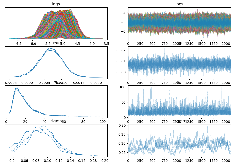Plots of the distribution (histogram/kernel density estimates) and sampled values

with model:
    trace = pm.sample(2100)

    az.plot_trace(trace)

Sanity Check

We can perform several sanity checks to ensure our simulation makes sense. To start, we provide an example of the returns we predicted in the test set. Next, we conduct a posterior predictive check to verify that the volatility we've learned accurately predicts the training data and also performs well on the test set.

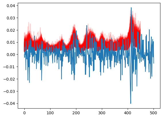True price and voltility

[plt.plot(1/np.exp(-trace.posterior['logs'].values[0,k]),color='r',alpha=.2) for k in range(1000,len(trace.posterior['mu'].values[0]))]
plt.plot(returns.values)

Cone of certainty

with model:
    pp = pm.sample_posterior_predictive(trace)

y_pred = pp["posterior_predictive"]["r"].values[0,:]
y_pred_mean = y_pred.mean(axis=0)

dfp = np.percentile(y_pred,[2.5,25,50,70,97.5],axis=0)

t = np.arange(0, len(returns.values))

plt.plot(returns.values,label='true value',alpha=0.5)
plt.plot(y_pred_mean, label='posterior mean')
plt.fill_between(train,dfp[0,:],dfp[4,:],alpha=0.5,color='gray',label='CR 95%')
plt.fill_between(train,dfp[1,:],dfp[3,:],alpha=0.4,color='blue',label='CR 50%')

plt.legend()

Projection and Bayesian Cone

Once we have trained the model, we will then use the data model to generate possible stock price trajectories. We will do this as follows:

Let $n$ represent the last day of the training set. For each ($\nu$,$\mu$,$\sigma$,$\log s_n$) which we sample from the posterior distribution, we will

1. Sample $\log s_{i+1} \sim \text{Normal}(\log s_{i}, \sigma^2)$ for $i > n$
2. Sample the change in the log stock price via $\log (S_{t+1}/S_t) \sim \text{StudentT}( \nu,\mu, sd=s_t)$
3. Repeat until we have done this for every day of the test set.

Next, we can add $\log(S_t)$ to each $\log(S_{t+1}/S_t)$, which gives us the log price for each day. If $S_t$ were representing a portfolio's cumulative return, the above process would apply in the same way.

import scipy.stats as stats

def generate_proj_returns(burn_in, trace, len_to_train):
   num_pred = 1000
   mod_returns = np.ones(shape = (num_pred,len_to_train))
   vol = np.ones(shape = (num_pred,len_to_train))
   for k in range(0,num_pred):
       nu = trace.posterior['nu'].values[1,burn_in+k]
       mu = trace.posterior['mu'].values[1,burn_in+k]
       sigma = trace.posterior['sigma'].values[1,burn_in+k]
       s = trace.posterior['logs'].values[1,burn_in+k][-1]
       for j in range(0,len_to_train):
           cur_log_return, s = _generate_proj_returns( mu,
                                                       s,
                                                       nu,
                                                       sigma)
           mod_returns[k,j] = cur_log_return
           vol[k,j] = s
   return mod_returns, vol

def _generate_proj_returns(mu,volatility, nu, sig):
   next_vol = np.random.normal(volatility, scale=sig)

   log_return = stats.t.rvs(nu, loc=mu, scale=1/np.exp(-1*next_vol))
   return log_return, next_vol

sim_returns, vol = generate_proj_returns(1000,trace,len(test))

prices = np.copy(sim_returns)
for k in range(0, len(prices)):
    cur = np.log(sp500[test[0]])
    for j in range(0,len(prices[k])):
        cur = cur + prices[k, j]
        prices[k, j] = cur

After calculating the log-stock price for each simulation, we will plot them and overlay the actual stock price for the test period. There are suggestions using the resulting cone to assess a trading algorithm: if the algorithm is overfitted or has any errors, its performance should deviate significantly from the cone's projection. If the actual value starts falling outside the cone, particularly if it happens suddenly, you should reconsider your strategy.

Even though stock prices might not always exhibit these issues, it can indicate that a stock is performing outside its expected volatility.

Below, we've plotted the projection in red and added a dotted black line to show the average linear trend, estimated using the mean of the posterior of $\mu$.

Projection and estimated trend

training_start = 400

slope = trace.posterior['mu'].values[2,1000:].mean()

trend = np.arange(0,len(test))*slope

ind = np.arange(len(train)+1,1+len(train)+len(test))
ind2 = np.arange(training_start,1+len(train)+len(test))

[plt.plot(ind, prices[j,:], alpha=.02, color='r') for j in range(0,1000)]
plt.plot(ind, trend + np.log(sp500)[len(train)+1],
            alpha=1,
            linewidth = 2,
            color='black',
            linestyle='dotted')

plt.plot(ind2,np.log(sp500)[ind2])

ax = plt.gca()
ax.set_ylim([7.4,7.8])
ax.set_xlim([training_start,len(sp500)-2])

Disclaimer

Naturally, the usual disclaimer applies: this method works until it doesn't. While it may not predict major market events, it can provide a baseline for evaluating various trading strategies and their potential.