Riemannian Geometry in Variational Autoencoders

Real data is often non-Euclidean. The space of 3D rotations, probability distributions on a statistical manifold, positions on a sphere--none of these have meaningful Euclidean distances.

Riemannian geometry provides tools for curved spaces. The central object is the metric tensor $\mathbf{G}(x)$, a smooth assignment of an inner product at each point. This allows defining lengths, angles, and shortest paths (geodesics) that respect the underlying geometry.

Often in literature the geometry is assumed. The goal here is to learn the geometry from data.

The Problem

Variational Autoencoders learn compressed representations by mapping high-dimensional inputs to a low-dimensional latent space. The latent coordinates are not identifiable--different training runs produce different representations encoding the same structure.

What is identifiable is the geometry. By equipping the latent space with a Riemannian metric derived from the decoder, distances remain consistent regardless of coordinate system.

Measure curve lengths in observation space, not latent space. Since curve length is invariant to reparametrization, so is distance. The coordinates are arbitrary, but the geometry is not.

Deriving the Metric

Given a decoder $f: \mathbb{R}^d \to \mathbb{R}^D$ and a curve $c(t)$ in latent space, define its length as the Euclidean length of its image:

$$ \mathrm{Length}(c) = \int_0^1 \left\lVert \frac{d}{dt} f(c(t)) \right\rVert dt $$

By the chain rule:

$$ \mathrm{Length}(c) = \int_0^1 \sqrt{\dot{c}_t^T \mathbf{J}_{c_t}^T \mathbf{J}_{c_t} \dot{c}_t} , dt = \int_0^1 \sqrt{\dot{c}_t^T \mathbf{G}_{c_t} \dot{c}_t} , dt $$

where $\mathbf{G} = \mathbf{J}^T \mathbf{J}$ is the Riemannian metric tensor and $\mathbf{J}$ is the Jacobian of the decoder. This is the pullback metric--pulling back the Euclidean metric from observation space via the decoder.

Implementation

We train a VAE with a 2D latent space on MNIST. The key is computing the Jacobian of the decoder efficiently.

import torch
import torch.nn as nn
import torch.nn.functional as F

class Encoder(nn.Module):
    def __init__(self, latent_dims):
        super(Encoder, self).__init__()
        self.linear1 = nn.Linear(784, 512)
        self.linear2 = nn.Linear(512, latent_dims)  # mean
        self.linear3 = nn.Linear(512, latent_dims)  # log-variance

    def forward(self, x):
        x = torch.flatten(x, start_dim=1)
        x = F.relu(self.linear1(x))
        mu = self.linear2(x)
        sigma = torch.exp(self.linear3(x))
        z = mu + sigma * torch.randn_like(mu)
        return z

class Decoder(nn.Module):
    def __init__(self, latent_dims):
        super(Decoder, self).__init__()
        self.linear1 = nn.Linear(latent_dims, 512)
        self.linear2 = nn.Linear(512, 784)

    def forward(self, z):
        z = F.relu(self.linear1(z))
        z = torch.sigmoid(self.linear2(z))
        return z.reshape((-1, 1, 28, 28))

Computing the Jacobian

For a network $f = f_L \circ f_{L-1} \circ \cdots \circ f_1$, the Jacobian is:

$$ \mathbf{J} = \mathbf{J}_{f_L} \mathbf{J}_{f_{L-1}} \cdots \mathbf{J}_{f_1} $$

For a linear layer $f(z) = Wz + b$, the Jacobian is $W$. For element-wise activations like ReLU or sigmoid, the Jacobian is diagonal with entries $\sigma'(z_i)$.

def jacobian_linear(W, x):
    """Jacobian of linear layer is just W, broadcasted for batch."""
    batch_size = x.shape[0]
    return W.unsqueeze(0).expand(batch_size, -1, -1)

def jacobian_sigmoid(x):
    """Jacobian of sigmoid is diag(sigmoid(x) * (1 - sigmoid(x)))."""
    s = torch.sigmoid(x)
    return torch.diag_embed(s * (1 - s))

def jacobian_relu(x):
    """Jacobian of ReLU is diag(x > 0)."""
    return torch.diag_embed((x > 0).float())

def decoder_jacobian(z, W1, b1, W2, b2):
    """Compute full Jacobian through decoder."""
    # Forward pass, keeping intermediates
    h1 = z @ W1.T + b1
    a1 = F.relu(h1)
    h2 = a1 @ W2.T + b2
    out = torch.sigmoid(h2)

    # Backward Jacobian chain
    J = jacobian_sigmoid(h2)           # (batch, 784, 784)
    J = J @ jacobian_linear(W2, a1)    # (batch, 784, 512)
    J = J @ jacobian_relu(h1)          # (batch, 784, 512)
    J = J @ jacobian_linear(W1, z)     # (batch, 784, 2)
    return J

The Metric Tensor

Once we have the Jacobian, the metric is straightforward:

def metric(z, decoder):
    J = decoder_jacobian(z, ...)  # (batch, 784, 2)
    G = J.transpose(1, 2) @ J     # (batch, 2, 2)
    return G

The volume element $\sqrt{\det(\mathbf{G})}$ measures how much the decoder stretches space at each point.

Visualizing the Latent Space

After training, each digit class clusters in a distinct region:

The 2D latent space. Each color represents a digit class (0-9).

Decoding points across the latent space:

Images decoded from a regular grid in latent space.

The Riemannian Metric

The metric tensor $\mathbf{G}(z) = \mathbf{J}(z)^T \mathbf{J}(z)$ varies across the latent space. We visualize its determinant (the local volume element):

The volume element $\sqrt{\det(\mathbf{G})}$ across latent space. Brighter regions indicate larger changes in observation space per unit movement in latent space.

The metric is higher where data is concentrated. The decoder packs more variation into small latent regions there, so the Jacobian has larger magnitude.

Geodesics

A geodesic is the shortest path between two points according to the Riemannian metric. The geodesic equation is:

$$ \ddot{c}^k + \Gamma^k_{ij} \dot{c}^i \dot{c}^j = 0 $$

where $\Gamma^k_{ij}$ are the Christoffel symbols derived from the metric. In practice, geodesics can be found by minimizing the curve energy:

$$ E[c] = \int_0^1 \dot{c}_t^T \mathbf{G}_{c_t} \dot{c}_t , dt $$

Geodesics connecting pairs of digit images. The paths curve to follow regions of high data density.

The geodesics bend around low-density regions rather than cutting through empty space.

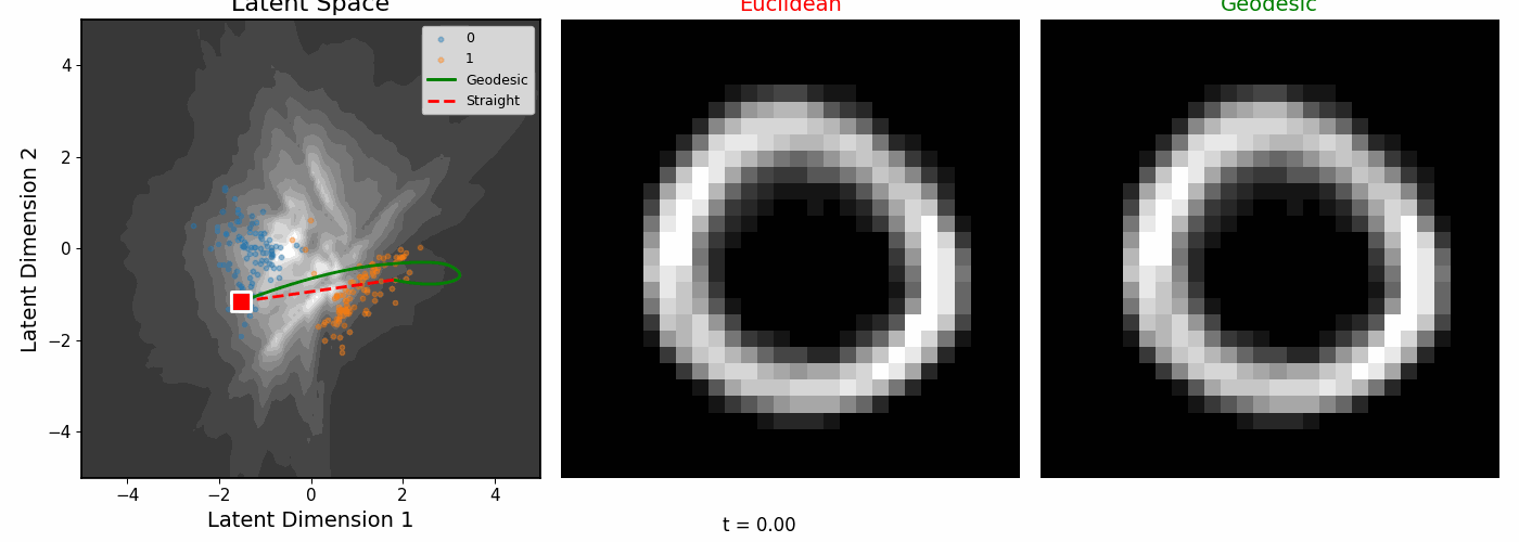
Euclidean vs Riemannian

The digit pairs on the left show the start (0) and end (1) images for each colored path. Middle: Euclidean interpolation. Right: Riemannian geodesics.

Interpolating between digits 0 and 1.

Distance Matrices

We can compute the average distance between all digit pairs using both metrics:

Average pairwise distances between digits. Left: Euclidean distance in latent space. Right: Geodesic distance.

The geodesic distances show more structure. Visually similar digits (like 4 and 9, or 3 and 8) have smaller geodesic/euclidean distances.

Conclusion

The VAE decoder has learned a Riemannian metric on the latent space. This metric encodes meaningful structure:

• Distances reflect similarity: Points close in geodesic distance produce similar images when decoded. Euclidean distance in latent space does not have this property.
• The metric captures data density: High metric values correspond to regions where data is concentrated. The decoder must represent more variation per unit of latent space there.
• Geodesics stay on the manifold: Shortest paths according to the learned metric avoid low-density regions, producing realistic interpolations.

There is a connection to density estimation. If we have data density $p(x)$ and want a metric under which the data is uniformly distributed, we seek $\sqrt{\det \mathbf{G}(x)}^{-1} \propto p(x)$--the volume element inversely proportional to density. See Lebanon (UAI 2003). The VAE decoder learns something similar automatically.

For a Gaussian VAE with observation noise $\sigma(z)$, the metric becomes:

$$ \mathbf{G}_z = \mathbf{J}_f(z)^T \mathbf{J}_f(z) + \mathbf{J}_\sigma(z)^T \mathbf{J}_\sigma(z) $$

The first term is the "mean" contribution, the second is an "uncertainty" term. Moving away from data increases uncertainty, making those regions longer according to the metric. This is exactly the behavior we want: the geometry penalizes paths through uncertain regions.