Having some fun with Julia and simulating a Wave packet in 2D.

Main Idea🔗

We will evolve the wavepacket in 2D by taking the tensor products between two 1D (x,y) spaces.

Wavepacket🔗

The wavepacket is expressed as a Gaussian:

\[\Psi(x) = \frac{\sqrt{\Delta x}}{\pi^{1/4}\sqrt{\sigma}} e^{i p_0 (x-\frac{x_0}{2}) - \frac{(x-x_0)^2}{2 \sigma^2}}\]

With the basis spanning the 1D space. And total state is represented by \(\Psi = \Psi_x \otimes \Psi_y\)

Hamiltonian🔗

The kinetic energy term is p_x^2/2 and p_y^2/2. The two-dimensional potential is a boundary with two slits.

function potential(x,y)
        if x > 20 && x < 25 && abs(y) > 1 && abs(y) < 5
                return 0
        elseif x > 20 && x < 25
                return 150
        elseif x > 48
                return 150
        else
                return 0
        end
end

I also use a gaussian potential:

potential(x,y) = exp(-(x^2 + y^2)/15.0)

Time Evolution🔗

At first, I had some trouble with installing DifferntialEquations.jl due to compilation errors for Arpack.jl. So I decided to just solve it manually by separating the real and imaginary components for the state, and then preforming the Discrete Laplace Operator for finite differences. Followed by adding the potential part. This is what I got: Double slit with Laplace

However, before I began working on visualization, Arpack.jl mysteriously compiled (probably because I switched to the official binary of Julia, rather than compiling my own). So I started exploring DifferntialEquations.jl. I then discovered QuantumOptics.jl which makes it pretty easy to simulate various quantum systems, so decided I should use it. It comes with a nice timeevolution.schroedinger which will evolve (integrate) the system.

Double Split starts with:

x0 = -5
y0 = 0
p0_x = 3.0
p0_y = 0.0
σ = 2.0

Guassian starts with:

x0 = -5
y0 = 0
p0_x = 1.5
p0_y = -.5
σ = 2.0

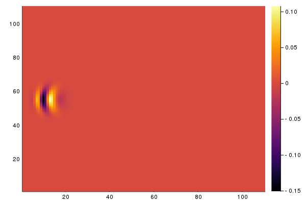
Results🔗

Julia has very nice support for plotting and animations. I abuse this here. Moreover, due to the Julia pre-compilation step, as long as you do not abuse the global space too much, the processing is rather quick.