Elliptic Curve Cryptography

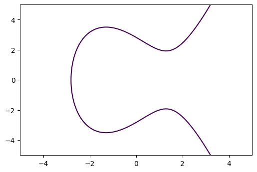
I dedicated some time to learn exactly what elliptic curves are and why they work in the first place. Here you'll find python codes that implement elliptic curves and some plots to help visualize what is going on. To begin, let's look at what an elliptic curve looks like over the real numbers!

import numpy as np
import matplotlib.pyplot as plt

Elliptic Curve over the Real Numbers

Example $y^2 = x^3 - 5x + 8$

def ecc_r(x):
    return x**3 - 5*x + 8

fig, ax = plt.subplots(dpi=100)
y, x = np.ogrid[-5:5:100j, -5:5:100j]
plt.contour(x.ravel(), y.ravel(), y**2 - ecc_r(x), [0])

<matplotlib.contour.QuadContourSet at 0x7ff64175c310>

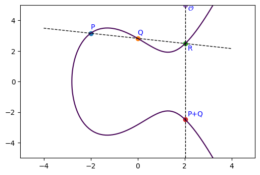
Adding points on Elliptic Curve

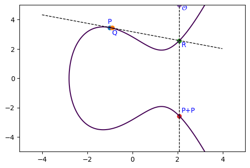
Suppose we have two points on $E$: $$P \approx (-2, 3.16)$$ $$Q \approx (-2, 2.82)$$

What is $P + Q$ on $E$? A good way to define this addition operation would be let the resulting point $E$ remain on the elliptic curve. Let's take a look at the following visualization where we draw tangential and vertical lines to define the addition.

# Points P and Q on E
P = np.array((-2, np.sqrt(ecc_r(-2))))
Q = np.array((0, np.sqrt(ecc_r(0))))

ax.scatter(*P)
ax.annotate('P', (P[0], P[1]+0.25), c='b')

ax.scatter(*Q)
ax.annotate('Q', (Q[0], Q[1]+0.25), c='b')

# Intersecting line
t = np.arange(-1, 3, 0.001)
line = np.array([(Q-P) * t_i + P for t_i in t])
ax.plot(line[:,0], line[:,1], linestyle='--', c='black', linewidth=1)

# Find points where the line intersects E
for l in line:
    if ecc_r(l[0]) > 0:
        if np.isclose(l[1], np.sqrt(ecc_r(l[0])), rtol=0.0001):
            R = l

# Plot the last point that intersected
ax.scatter(*R)
ax.annotate('R', (R[0]+0.1, R[1]-0.45), c='b')

# Draw vertical line, and the new point which is our sum P+Q
ax.axvline(R[0], linestyle='--', c='black', linewidth=1)
ax.scatter(R[0], -R[1])
ax.annotate('P+Q', (R[0]+0.1, -R[1]+0.25), c='b')

# Draw the point at infinity to have 3 points of intersection for vertical line
ax.scatter(R[0], ax.get_ylim()[1])
ax.annotate(r'$\mathcal{O}$', (R[0]+0.1, ax.get_ylim()[1] - 0.35), c='b')

fig

Adding a Point To Itself on $E$

Now how do we add a point $P$ with itself? There are multiple lines that intersect $P$...

Let's imagine our second point $Q$ approaches to $P$: $Q \to P$. Well that's the derivative at the point P!

Let's take: $$P = (-1, 3.16)$$

fig = plt.figure(dpi=100)

# The point P
P = np.array((-1, np.sqrt(ecc_r(-1))))

plt.scatter(*P)
plt.annotate('P', (P[0]-0.1, P[1]+0.25), c='b')
plt.scatter(P[0]+0.1, P[1])
plt.annotate('Q', (P[0]+0.1, P[1]-0.5), c='b')


# Plot ECC
y, x = np.ogrid[-5:5:1000j, -5:5:1000j]
plt.contour(x.ravel(), y.ravel(), y**2 - ecc_r(x), [0])

# Dervative to find tangent point
def d_dx_e(x):
    n = 3 * x ** 2 - 5
    d = 2 * np.sqrt(x**3 - 5 * x + 8)
    return n / d

# Plot the tangent to P
t = np.arange(-4, 4, 0.01)
def y_intercept(x_i, m):
    return m * (x_i - P[0]) + P[1]

line = y_intercept(t, d_dx_e(P[0]))
plt.plot(t, line, linestyle='--', c='black', linewidth=1)

# Get the intersection points of E with tangent line
temp = [ecc_r(t_i) if ecc_r(t_i) > 0 else 0 for t_i in t]
idx = np.argwhere(np.diff(np.sign(np.sqrt(temp) - line))).flatten()[-1:][0]

R = t[idx], line[idx]
plt.scatter(*R)
plt.annotate('R', (R[0]+0.1, R[1]-0.45), c='b')

# Draw vertical line
plt.axvline(t[idx], linestyle='--', c='black', linewidth=1)

plt.scatter(R[0], -R[1])
plt.annotate('P+P', (R[0]+0.1, -R[1] + 0.25), c='b')


# Draw the point at infinity to have 3 points of intersection for vertical line
plt.scatter(R[0], ax.get_ylim()[1])
plt.annotate(r'$\mathcal{O}$', (R[0]+0.1, ax.get_ylim()[1] - 0.35), c='b')

Text(2.1799999999998705, 4.65, '$\\mathcal{O}$')

Formula for Point Addition

Suppose we want to add two points: $P_1 = (x_1, y_1)$ and $P_2 = (x_2, y_2)$ on the Elliptic curve: $$E: y^2 = x^3 + Ax + B$$

Let the line connecting $P_1$ to $P_2$ be $$L: y = \lambda x + \nu$$

From the examples above, we can write the slope of $L$ by:

$$\lambda = \begin{cases} \frac{y_2 - y_1}{x_2 - x_1} & P_1 \neq P_2 \\ \frac{3x_1^2 + A}{2y_1} & P_1 = P_2 \end{cases}$$

And the y-intercept of $L$: $$\nu = y_1 - \lambda x_1$$

To find the intersection of the Elliptic curve $E$ and $L$ we need to solve: $$(\lambda x + \nu)^2 = x^3 + Ax + B$$

Since we already know that $x_1$ and $x_2$ are solutions, we can find the third solution $x_3$ by comparing the both sides:

$$x^3 + Ax + B - (\lambda x + \nu)^2 = (x-x_1)(x-x_2)(x-x_3)$$

So for example, if we look at $x^2$ terms this gives $-\lambda^2 = -x_1 - x_2 - x_3$ and so $x_3 = \lambda^2 - x_1 - x_2$. Computing $y_3$ then tells us that:

$$P_1 + P_2 = (x_3, -y_3)$$

Summary

From the formula we can derive the following:

• If $P_1 \neq P_2$ and $x_1 = x_2$ then $P_1 + P_2 = \mathcal{O}$

• If $P_1 = P_2$ and $y_1 = 0$ then $P_1 + P_2 = 2P_1 = \mathcal{O}$

• If $P_1 \neq P_2$ (and $x_1 \neq x_2$) let $$\lambda = \frac{y_2 - y_1}{x_2 - x_1} \quad \nu = \frac{y_1x_2 - y_2x_1}{x_2 - x_2}$$

• If $P_1 = P_2$ (and $y_1 \neq 0$) let $$\lambda = \frac{3x_1^2 + A}{2y_1} \quad \nu = \frac{-x^3 + Ax + 2B}{2y}$$ Then $P_1 + P_2 = (\lambda^2 - x_1 - x_2, -\lambda^3 + \lambda(x_1 + x_2) - \nu)$

Observations

$$x(P_1 + P_2) = \left( \frac{y_2 - y_1}{x_2 - x_1}\right)^2 - x_1 - x_2$$ and for $P = (x,y)$ then, $$x(2P) = \frac{x^4 - 2Ax^2 - 8Bx +A^2}{4(x^3 + Ax + B)}$$

Point at Infinity

The special $\mathcal{O}$ that has been showing up is the point at infinity. It's a special point which doesn't necessarily live on the curve, but instead represents an imaginary 3rd point so that our vertical line has a reasonable interpreation. So, for example, $P + \mathcal{O} = Q$. This means points $P$ and $\mathcal{O}$ formed a line and the final point on that line is $Q$.

Poincare Theorem

If points $P$ and $Q$ have coordinates in a field $K$, then $P+Q$ and $2P$ also have coordinates in $K$. More formally:

• Let $K$ be a field and suppose that an elliptic curve E is gen by an equation: $y^2 = x^3 + Ax + B$ with $A,B \in K$.
• Let $E(K)$ denote the set of points of $E$ with coordinates in $K$: $E(K) = {(x,y)\in E: x,y \in K} \cup \mathcal{O}$
• Then $E(K)$ is a subgroup of the group of all points of $E$

Lets use a different field instead of the real numbers (and keep using the formulas we derived for real numbers under the new field operations)!

Elliptic Curves over a Finite Field

Of course using real numbers are not that great to use when we want to do things with computers. But worry not, we can instead use a different field. A finite field is also called a Galois field and is usually denoted $GF(k)$ or $\mathcal{F}_k$. The order (or the number of elements) of a finite field is always prime or a power of a prime.

Prime Field

$GF(p$) is called the Prime Field of order $p$ where $p$ is prime, and the elements are ${0, 1, ..., p-1}$.

Operations over the Finite Field $GF(p)$

We can perform addition, subtraction, and multiplication as we usually do on the integers, just now under modulo $p$. E.g. in $GF(5)$, $4 + 3 = 7$ mod $5$ = $2$ mod $5$. And likewise, $4 \cdot 3 = 4 + 4 + 4$ mod $5$ = $2$ mod $5$.

Now, in order to do division of a number $x \in GF(p)$ we need to compute the inverse of $x$, denoted as $x^{-1}$. For the finite field, we can use the Extended Euclidean algorithm to compute the inverse!

# Extended Euclidean Algorithm for finding inverse of x mod p
def eea(x, p, debug=False):
    # Quotient
    q = int(p / x)
    # Remainder
    r = r_old = p % x

    q_s = [q]
    a_s = [0, 1]
    i = 0
    while True:
        if debug:
            print(f'{q * x + r} = {q} * {x} + {r}')
        if i > 1:
            a_i = (a_s[i-2] - a_s[i-1] * q_s[i-2]) % p
            a_s.append(a_i)
        if r == 0:
            if r_old != 1:
                assert "No inverse"
            i = i + 1
            break
        r_old = r
        q = int(x / r)
        q_s.append(q)
        r = x % r
        x = r_old
        i = i + 1

    a_i = (a_s[i-2] - a_s[i-1] * q_s[i-2]) % p
    return a_i

So now for $\frac{x}{y}$ = $x * \frac{1}{y}$ = $x * y^{-1}$, where $x,y \in GF(p)$ we need to compute the inverse of y. Consider the example below in $GF(37)$, where we compute: $$\frac{15}{29} = 15 \cdot 29^{-1} = 15 * 23 \text{ mod } 37 = 12$$

But in the special case when $x \in GF(p)$ where $p$ is prime, the inverse of $x$ is just $x^{p-2}$.

Great, but now let us also look at finding the square root. Taking the normal square root over the real numbers will not work. But since we know the finite set of numbers in $GF(p)$ we also know all the possible $x^2$, so we can search for when $y = x^2$ for a given $x$. This also means that taking the $\sqrt{y}$ where $y \in GF(p)$ will have either 0 or 2 solutions.

inverse = eea(29, 37, debug=True)
print(f"Inverse: {inverse}")
print(f"Check: {29} * {inverse} mod {37}: {29 * inverse % 37}")
print(f"{15} * {inverse} mod {37}: {15 * inverse % 37}")

37 = 1 * 29 + 8
29 = 3 * 8 + 5
8 = 1 * 5 + 3
5 = 1 * 3 + 2
3 = 1 * 2 + 1
2 = 2 * 1 + 0
Inverse: 23
Check: 29 * 23 mod 37: 1
15 * 23 mod 37: 12

So great, we have shown the inverse of 29 is 23. But there's actually a special case in which the inverse can be found using: $x^{p-2} mod p$ if $p$ is prime. In general however, we require the extended euclidan algorithm since in general we can have a $GF(p^n)$.

Implementing Elliptic Curve over Finite Field

def ecc(x, p, A, B):
    assert (4*A**3 + 27*B**2) % p!= 0
    return (x**3 + A*x + B) % p

# Find the elements in x^2 that are equal to elements in y^2, which in finite field is to find sqrt
def sqrt_f(x, y2, p):
    x2 = x**2 % p
    y = [(i, *y_i) for i, y_i in enumerate([np.where(y2_i == x2)[0] for y2_i in y2]) if y_i.size > 0]
    return y

Functions to compute the sum of points on Elliptic Curve. Also check these implementations. Note, these are directly the formula derived above just now using the finite field operations under the modulo $p$.

def get_2P(P, p, A, B):
    x,y = P
    
    lam = (3 * x**2 + A) * eea(2 * y, p) % p
    nu = (-x**3 + A*x + 2*B) * eea(2 * y, p) % p
    # n = (x**4 - 2*A*x**2 - 8*B*x + A**2) % p
    # d = (4 * (x ** 3 + A * x + B)) % p
    # d = eea(d, p)
    return (lam**2 - 2*x) % p, (-lam**3 + 2*lam*x - nu) % p
    # return n * d % p, ecc(n * d % p, p, A, B)

def get_PQ(P, Q, p, A, B):
    x1,y1 = P
    x2,y2 = Q

    lam = (y2 - y1) * eea((x2 - x1) % p, p) % p
    nu = (y1*x2 - y2*x1) * eea((x2 - x1) % p, p) % p

    return (lam**2 - x1 - x2) % p, (-lam**3 + lam*(x1 + x2) - nu) % p

def sum_on_E(P, Q, p, A, B):

    # We have a point at infinity
    if (P == 0):
        return Q
    if (Q == 0):
        return P
    if (P == Q):
        if P[0] == 0:
            # Point at infinity
            return 0
        val = get_2P(P, p, A, B)
        return val
    else:
        if P[0] == Q[0]:
            return 0

        val = get_PQ(P, Q, p, A, B)
        return val

Example

Let the prime field have order: $p=37$.

And let our curve be: $$E: y^2 = x^3 - 5x + 8, \text{ mod } p$$

The elements in this field/group are: ${0, 1, 2, ..., 36}$

With that in mind, let us plot this curve

# Order
p = 37
x = np.array(range(0, p))

A = -5
B = 8

x2 = x**2 % p
y2 = ecc(x, p, A, B)

# Compute the sqrt of the elliptic curve for plotting
y = sqrt_f(x, y2, p)

fig = plt.figure(dpi=100)
for y_p in y:
    [plt.scatter(y_p[0], i, c='b') for i in y_p[1:]]

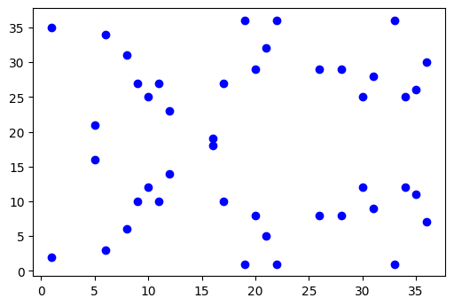
The number of points generated for $E(GF_{37})$ =

# Number of points and +1 for point at infinity
len(sum([y_p[1:] for y_p in y], ())) + 1

45

And the points look like:

print(*['[x:{}, y:{}]'.format(y_p[0], y_p[1:]) for y_p in y])

[x:1, y:(2, 35)] [x:5, y:(16, 21)] [x:6, y:(3, 34)] [x:8, y:(6, 31)] [x:9, y:(10, 27)] [x:10, y:(12, 25)] [x:11, y:(10, 27)] [x:12, y:(14, 23)] [x:16, y:(18, 19)] [x:17, y:(10, 27)] [x:19, y:(1, 36)] [x:20, y:(8, 29)] [x:21, y:(5, 32)] [x:22, y:(1, 36)] [x:26, y:(8, 29)] [x:28, y:(8, 29)] [x:30, y:(12, 25)] [x:31, y:(9, 28)] [x:33, y:(1, 36)] [x:34, y:(12, 25)] [x:35, y:(11, 26)] [x:36, y:(7, 30)]

An observation is that there are nine points of order dividing three, so this set of numbers has an interesting abstract group formed by two cyclic groups $C$: $$E(GF_{37}) \cong C_3 \times C_{15}$$

In fact, any $E(GF_p)$ will always be a cyclic group or the product of two cyclic groups.

Order and Cofactor of Elliptic Curve

In this example, the order (number of elements including point at infinity) of our Elliptic Curve is $n=45$. Moreover we can write the order in relation to the number of cyclic groups $h$ (cofactor),and the number of points in those cyclic groups $r$.

$$ n = h \cdot r$$

Examples:

• secp256k1 has h=1
• Curve25519 has h=8
• Curve448 has h=4

Computing $mP$

We will see later that we would like to compute the multiples of $mP = P + P + ... + P \in E(GF_p)$, for very large values of $m$. This can be done in $O(log m)$ steps by expanding $m$ in binary: $$m = m_0 + m_1 \cdot 2 + ... + m_r \cdot 2^r$$

Then $mP$ is computed as: $$mP = m_0 P + m_1 \cdot 2P + m_2 \cdot 2^2 P + ... + m_r \cdot 2^r P$$ where $2^k P = 2\cdot 2 ... 2P$ requires only k doublings. Hence on average, it takes $log_2(m)$ doublings and $\frac{1}{2}log_2(m)$ additions to compute $mP$.

We can even consider high-order expansion and see that we can reduce the number of operations. So, for ternary, we have $\frac{1}{3} log_2(m)$ additions.

def compute_mP(m, P, p, A, B):
    # Get binary string for m
    m_binary = "{:b}".format(m)

    doubling_P = list(range(len(m_binary)))
    doubling_P[0] = P
    for i in doubling_P[1:]:
        doubling_P[i] = sum_on_E(doubling_P[i-1], doubling_P[i-1], p, A, B)
    # print

    # Get all non-zero m_i * 2^i P
    to_compute = [doubling_P[i] for i in range(len(m_binary)) if m_binary[::-1][i] == '1']
    # print(to_compute)
    
    # Get the sum
    result = to_compute[0]
    for P_2i in to_compute[1:]:
        result = sum_on_E(result, P_2i, p, A, B)
    return result

This method is not very symmetric in it's computation. We only preform an operation when $m_i = 0$, which makes it prone to timing/power attacks! An alternative that is symmetric: Montgomery ladder

Let us take a look at what happens when you preform $mP$ where $m \in [1, 16]$ and $P = (6,3)$. We can see it's cyclic!

fig = plt.figure(dpi=100)

for y_p in y:
    [plt.scatter(y_p[0], i, c='b') for i in y_p[1:]]

P = (6,3)
for r in range(1,17):
    R = compute_mP(r, P, p, A, B)
    if R == 0:
        continue
    plt.scatter(*R, c='r', alpha=0.4)
    plt.annotate(f'{r+1}', (R[0]+0.25, R[1]), c='r')

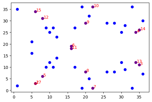
Namely we see that our point $P = 17P$. And moreover, we generated 14+1 (including point at infinity) points that live on the curve! Let's see what happens if we choose other points.

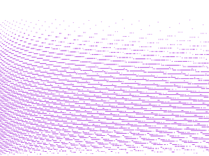
fig = plt.figure(dpi=100)

for y_p in y:
    [plt.scatter(y_p[0], i, c='b') for i in y_p[1:]]

cmap = plt.cm.get_cmap('hsv', len(y))

# Transform our points from the curve into one big stack of (x,y)

for i, y_i in enumerate(y):
    P = (y_i[0], y_i[1])
    group = []
    for r in range(1,45):
        R = compute_mP(r, P, p, A, B)
        if R == 0:
            break
        group.append(R)
    group = np.array(group)
    plt.scatter(group[:,0], group[:, 1], c=[cmap(i) for _ in range(len(group))], alpha=0.5, label="{} - {}".format(P, len(group)+1))
    # for r, R in enumerate(group):
    #     plt.annotate(f'{r+1}', (R[0]+0.25, R[1]), c=cmap(i))

plt.legend(loc='center left', bbox_to_anchor=(1, 0.5))

<matplotlib.legend.Legend at 0x7ff63ed64fa0>

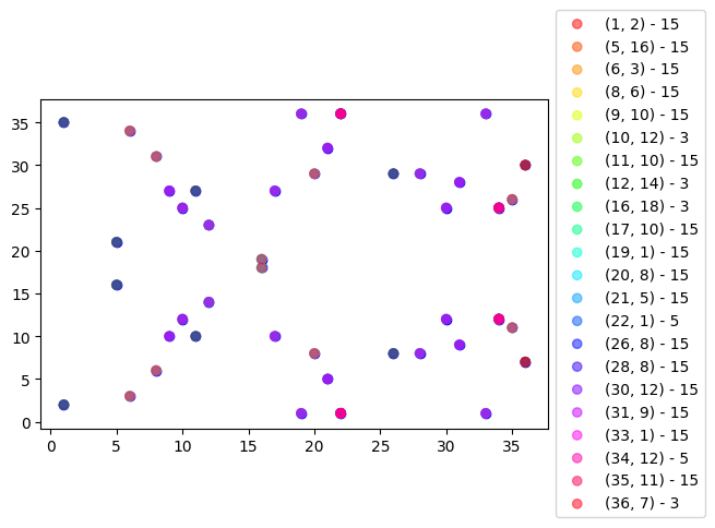
Generator Point in E and Security

We see that by multipling a point $P$ by itself gives us other points on the curve. If that point $P$, with multipling itself, generates all the points in it's subgroup then the point is called the generator $G$. When we multiply $G$ by number $m \in [0, r]$, we can get a subgroup of other points on the curve. This $r$ is called the order. The order $r$ is actually equal to the total number of all possible private keys. So it is important that a carefully selected point $G$ gives a large enough subgroup of the curve, otherwise there will be a possibility for a small-subgroup attacks. So in our example, we would want to choose a point that generates the cyclic group with order $15$, not the one for order $3$.

Public and Private Keys

We have seen that we can generate several points on the curve by picking a point $G$ and multiplying it by a number $m \in [1, r]$ which gives use points $P = mG$. Moreover, we have seen that figuring out what $mG$ is, can be done in $log_2(m)$ time. However, the reverse is not true: figuring out what $m = P / G$ is slow. For this reason, given an Elliptic Curve over a field $GF(p)$:

• $G$ is a fixed point chosen for that curve
• $m$ is the private key
• $P = mG$ is the public key

Using the example above, we fix $G = (6,3)$ and then let

• $m = 13$ be the private key
• $mG = 13\cdot(6,3) = (35, 26) = P$ be our public key

Curve Strength

Let our private key $m$ have size $k$. Then the fast known algorithm needs $\sqrt{k}$ steps to solve for $m$. So a large $m$ is important, which requires a large field size to generate the curve on, and also requires that the subgroup we find is big.

In order to implement k-bit security strength, a 2k-bit curve is needed. So for example, secp256k1 has ~128-bit security, since the field size it generates is 256 and it only has one subgroup, so any point you pick as the generator will create a subgroup with size 256.

Usually, the subgroup will be smaller than the field size. So on average the number of steps required for the algorithm is closer to $0.886\sqrt{k}$.

Real-world example: secp256k1

Wouldn't recommend using this curve in real practice...

https://safecurves.cr.yp.to/ list safe/unsafe curve parameters... so probably follow that

Anyway, let's just see how ECC works with some real curves. I took the parameters from SEC2

p = int('0xfffffffffffffffffffffffffffffffebaaedce6af48a03bbfd25e8cd0364141', 16)
A = 0
B = 7

# The generator point
G = (int('0x79be667ef9dcbbac55a06295ce870b07029bfcdb2dce28d959f2815b16f81798', 16),
     int('0x483ada7726a3c4655da4fbfc0e1108a8fd17b448a68554199c47d08ffb10d4b8',16))

# How many points in the curve:
n = int('0xfffffffffffffffffffffffffffffffebaaedce6af48a03bbfd25e8cd0364141', 16)

# How many subgroups in the curve
h = 1

# My random private key
k = int('0x51897b64e85c3f714bba707e867914295a1377a7463a9dae8ea6a8b914246319', 16)

# Generate point on E
P = compute_mP(k, G, p, A, B)

# Remember that the curve is symmetric, so we can pick one of the points
# P_compressed = '0' + str(2 + P[1] % 2) + str(hex(P[0])[2:])

print('Private Key: {}'.format(hex(k)[2:]))
print('Public Key: {}'.format(str(P[1] %2) + str(hex(P[0])[2:])))

Private Key: 51897b64e85c3f714bba707e867914295a1377a7463a9dae8ea6a8b914246319
Public Key: 19d925d49eeec2186a6d3c50ba38246c441ef0ea3c1f47bd5158b8972a2816562